251211_BootCamp Day 39_선형회귀
2025. 12. 11. 20:12ㆍTIL
import pandas as pd
import numpy as np
import matplotlib.pyplot as plt
import seaborn as sns
# Scikit-learn에서 제공하는 샘플 데이터셋 중 하나인 diabetes 불러오기
from sklearn.datasets import load_diabetes
# Scikit-learn의 linear model 중 하나인 LinearRegression(선형회귀) 모델 불러오기
from sklearn.linear_model import LinearRegression
lr = LinearRegression
diabetes = load_diabetes()
# 불러온 diabetes 데이터 확인하기
# sklearn.utils._bunch.Bunch라는 처음 보는 데이터타입
# key와 value로 구성되어 있음 (dictionary와 유사한 형태)
# data : 샘플 데이터 (Numpy 배열 형태)
# target : Label 데이터 (Numpy 배열 형태)
# feature_names : data의 각 column 이름
# target_names : target(label 데이터)의 각 column 이름
diabetes
diabetes.keys()
diabetes.feature_names
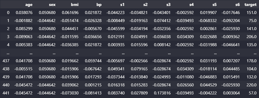
# dataset의 feature_names와 target을 컬럼으로 하고, 내부 데이터는 data, target으로 하는 데이터프레임 생성
# 모델에 넣기 위해 데이터프레임 형태로 바꿔줘야 한다.
# np.c_ : 두 Numpy 배열을 가로 방향으로 합치는 함수
df = pd.DataFrame(data=np.c_[diabetes.data, diabetes.target], columns=diabetes.feature_names + ['target'])

# 히스토그램을 통한 데이터 분포 살펴보기
# diabetes의 각 컬럼 별로 분포가 어떻게 되어 있는지 확인할 수 있다.
df.hist(bins=20, figsize=(10, 10), color='blue')
plt.tight_layout()
plt.show()
# 변수 간 상관관계를 히트맵으로 확인할 수 있다.
corr_matrix = df.corr()
plt.figure(figsize=(10, 8))
# np.ones_like : corr_matrix와 똑같은 크기의 행렬을 만드는데, 내용을 모두 bool(True)로 채운다.
# True  True  True
# True  True  True
# True  True  True
# np.triu : 대각선과 그 위쪽만 남기고, 나머지는 0(False)으로 바꾼다.
# True  True  True
# False True  True
# False False True
mask2 = np.triu(np.ones_like(corr_matrix, dtype=bool))
# 히트맵의 mask에 해당 내용을 넣으면, True인 부분은 가려지게 된다.
sns.heatmap(corr_matrix, annot=True, cmap='RdYlGn', linewidths=0.5, mask=mask2, fmt='.2f')
plt.title("Heatmap Using Seaborn Library")
plt.show()
# 독립변수 (X) : BMI
# 종속변수 (Y) : 당뇨병 진행 단계 (target)
# 독립변수와 종속변수의 관계를 보기 위해 산점도로 시각화
sns.scatterplot(x='bmi', y='target', data=df, color='#D2C1D2', marker='o', edgecolor='black')
plt.xlabel("BMI")
plt.ylabel("Progression of Diabetes")
plt.title("Relationship Between Progression of Diabetes & BMI")
plt.show()
diabetes = load_diabetes()
# 선형회귀모델에 적용하기 위한 X, y 설정
X = df.bmi.values
y = df.target.values
# 단순선형회귀 모델 선언
model = LinearRegression()
# 머신러닝 모델에는 2차원 형태의 배열을 사용해야 하기 때문에 1차원(series)인 X를 2차원(dataframe) 형태로 바꿔줘야 한다.
X = X.reshape(-1, 1)
# 선언한 단순선형회귀 모델 학습 (fit)
model.fit(X, y)
# 만들어진 단순선형회귀 모델의 회귀계수와 y절편 확인
# 회귀계수 : 949.43526.., y절편 : 152.13348...
# 회귀식 : y = 949.43526x + 152.13348
model.coef_[0], model.intercept_
# 만들었던 산점도에 회귀선 추가하기
sns.scatterplot(x='bmi', y='target', data=df, color='green', marker='*')
plt.plot(X, model.predict(X), color='red', linewidth=2)
plt.xlabel("BMI")
plt.ylabel("Progression of Diabetes")
plt.title("Relationship Between Progression of Diabetes & BMI")
plt.show()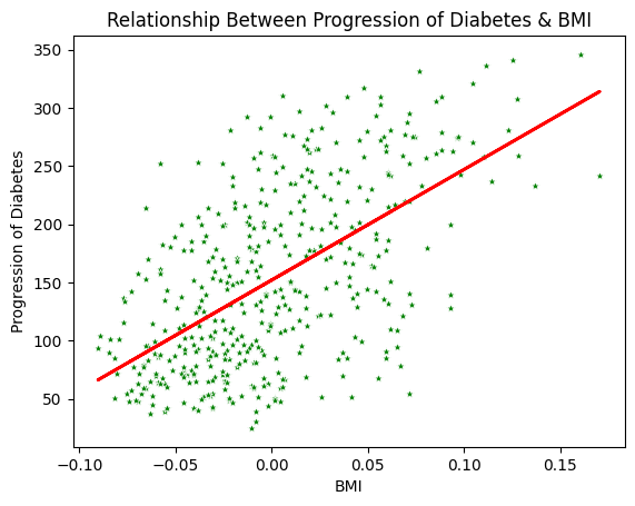
# OLS를 이용한 회귀분석 결과 해석하기
# R-squared, Adj. R-squared : 결정계수
# F-statistic, Prob(F-statistic) : F-검정 결과, F-검정 p-value
# t, P>|t| : t검정 결과, t검정 p-value
import statsmodels.api as sm
results = sm.OLS(y, sm.add_constant(X)).fit()
results.summary()
# Standard Erors assume that the covariance matrix of the errors is correctly specified
# OLS가 잔차의 등분산성과 무자기상관성이 만족된다는 가정 하에 표준오차를 계산했다는 의미
# 만약 데이터가 그렇지 않다면, OLS의 결과를 믿을 수 없다는 뜻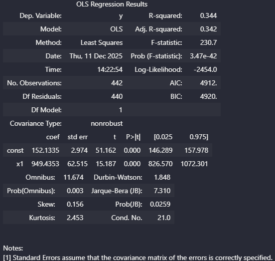
해석 결과
R-quared=0.344 : 이 회귀분석 모델은 34% 정도 데이터를 설명할 수 있다.
Prob(F-statistic)=3.47e-42 : 회귀식이 회귀분석 모델 전체에 대해 통계적으로 의미가 있다
P>|t|=0.000 : 각 변수가 종속변수에 미치는 영향이 유의한지 판단 -> 0.05보다 작으므로 X(bmi)는 target(당뇨병 진행 정도)를 설명하는 데 유의하다.
# 잔차 (residual)의 분포 확인하기
y_pred = model.predict(X)
residuals = y - y_pred
plt.figure(figsize=(10, 6))
sns.histplot(residuals, kde=True, color='blue')
plt.axvline(0, color='red', linestyle='--')
# QQ-plot 확인하기
import scipy.stats as stats
plt.figure(figsize=(10, 6))
stats.probplot(residuals.flatten(), dist="norm", plot=plt)
'TIL' 카테고리의 다른 글
| 251215_BootCamp Day 41_XGBoost, LightGBM (2) | 2025.12.15 |
|---|---|
| 251212_BootCamp Day 40_분류분석 (0) | 2025.12.12 |
| 251210_BootCamp Day 38_기초 통계학 (2) (1) | 2025.12.10 |
| 251209_BootCamp Day 37_기초 통계학 (1) (2) | 2025.12.09 |
| 251208_BootCamp Day 36_표준화와 정규화 (0) | 2025.12.08 |